capezza2020

Control charts for monitoring a scalar quality characteristic adjusted for by the effect of functional covariates

In this vignette we show how to use the funcharts package to apply the methods proposed in Capezza et al. (2020) to build control charts for monitoring scalar quality characteristic adjusted for by the effect of functional covariates, based on scalar-on-function regression. Let us show how the funcharts package works through an example with the dataset air, which has been included from the R package FRegSigCom and is used in the paper of Qi and Luo (2019). The authors propose a function-on-function regression model of the NO2 functional variable on all the other functional variables available in the dataset. In order to show how the package works, we consider a scalar-on-function regression model, where we take the mean of NO2 at each observation as the scalar response and all other functions as functional covariates.

First of all, starting from the discrete data, let us build the multivariate functional data objects of class mfd, see vignette("mfd").

library(funcharts)
data("air")
fun_covariates <- names(air)[names(air) != "NO2"]
mfdobj_x <- get_mfd_list(air[fun_covariates], grid = 1:24)

Then, we extract the scalar response variable, i.e. the mean of NO2 at each observation:

y <- rowMeans(air$NO2)

In order to perform the statistical process monitoring analysis, we divide the data set into a phase I and a phase II dataset.

rows1 <- 1:300
rows2 <- 301:355
mfdobj_x1 <- mfdobj_x[rows1]
mfdobj_x2 <- mfdobj_x[rows2]
y1 <- y[rows1]
y2 <- y[rows2]

Scalar-on-function regression

We can build a scalar-on-function linear regression model where the response variable is a linear function of the multivariate functional principal components scores. The principal components to retain in the model can be selected with selection argument. Three alternatives are available (default is variance):

• if “variance” (default), the first M multivariate functional principal components are retained into the MFPCA model such that together they explain a fraction of variance greater than tot_variance_explained,
• if “PRESS”, each j-th functional principal component is retained into the MFPCA model if, by adding it to the set of the first j-1 functional principal components, then the predicted residual error sum of squares (PRESS) statistic decreases, and at the same time the fraction of variance explained by that single component is greater than single_min_variance_explained. This criterion is used in Capezza et al. (2020).
• if “gcv”, the criterion is equal as in the previous “PRESS” case, but the “PRESS” statistic is substituted by the generalized cross-validation (GCV) score.

Here, we use default values:

mod <- sof_pc(y = y1, mfdobj_x = mfdobj_x1)

As a result you get a list with several arguments, among which the original data used for model estimation, the result of applying pca_mfd on the multivariate functional covariates, the estimated regression model. It is possible to plot the estimated functional regression coefficients, which is also a multivariate functional data object of class mfd:

plot_mfd(mod$beta)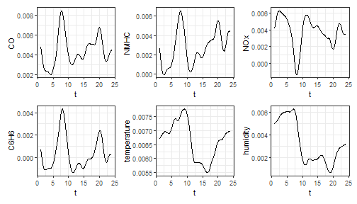

Moreover bootstrap can be used to obtain uncertainty quantification:

plot_bootstrap_sof_pc(mod, nboot = 10)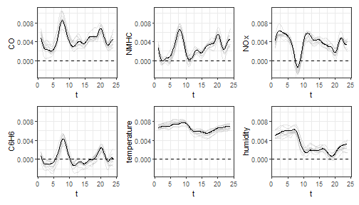

Control charts

We can build the regression control chart to monitor the scalar response, as performed in Capezza et al. (2020). The function regr_cc_sof provides a data frame with all the information required to plot the desired control charts. Among the arguments, you can pass the arguments y_tuning and mfdobj_x_tuning set, that are not used for model estimation/training, but only to estimate control chart limits. If these arguments are not provided, control chart limits are calculated on the basis of the training data. The arguments y_new and mfdobj_x_new contain the phase II data set of observations of the scalar response and the functional covariates to be monitored, respectively. The function plot_control_charts returns the plot of the control charts.

cclist <- regr_cc_sof(object = mod,
                      y_new = y2,
                      mfdobj_x_new = mfdobj_x2)
plot_control_charts(cclist)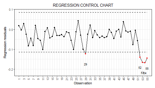

References

• Capezza C, Lepore A, Menafoglio A, Palumbo B, Vantini S. (2020) Control charts for monitoring ship operating conditions and CO2 emissions based on scalar-on-function regression. Applied Stochastic Models in Business and Industry, 36(3):477–500. https://doi.org/10.1002/asmb.2507
• Qi X, Luo R. (2019). Nonlinear function-on-function additive model with multiple predictor curves. Statistica Sinica, 29:719–739. https://doi.org/10.5705/ss.202017.0249