Scalar-on-Function Regression Control Chart — regr_cc

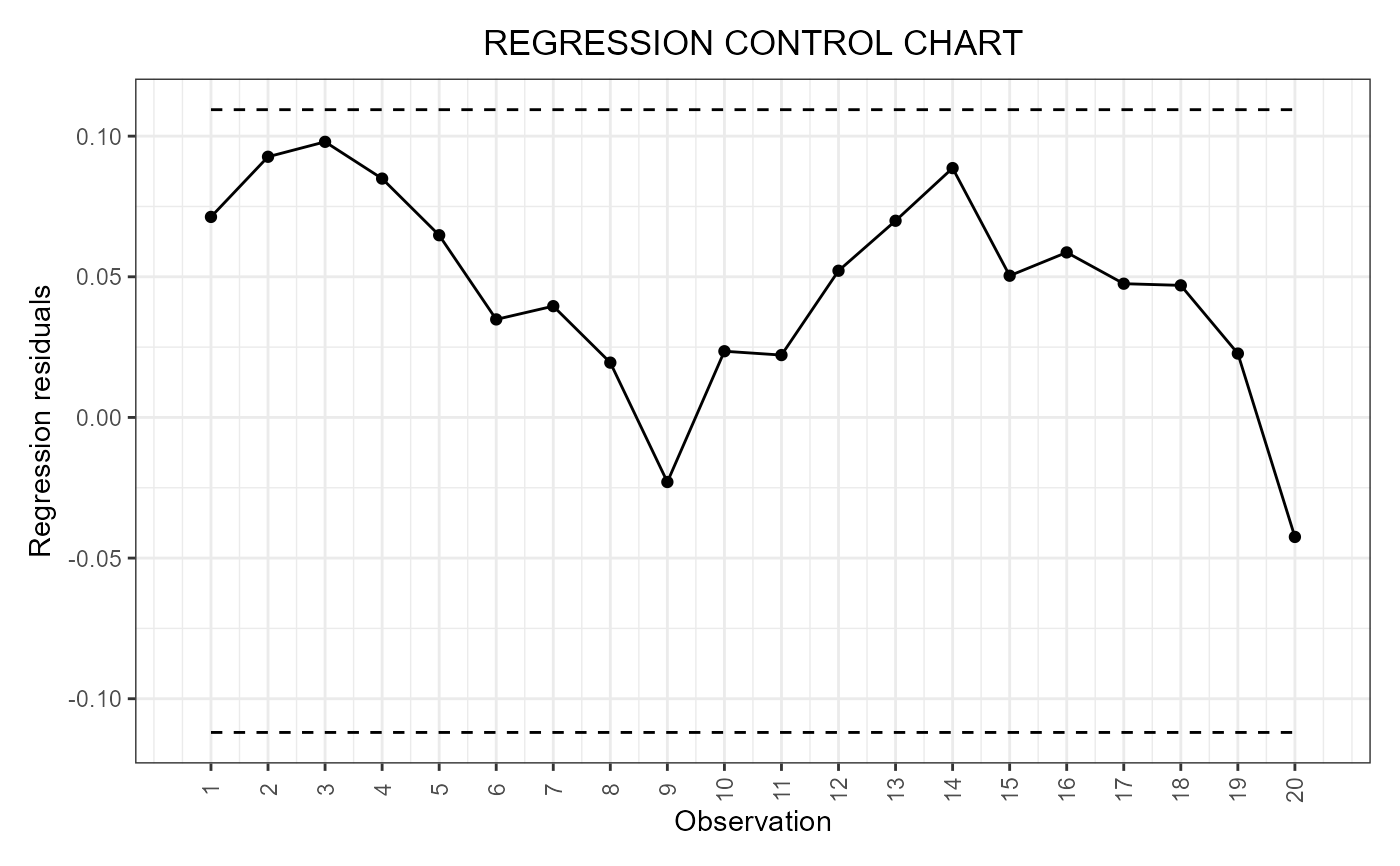
This function is deprecated. Use regr_cc_sof. This function builds a data frame needed to plot the scalar-on-function regression control chart, based on a fitted function-on-function linear regression model and proposed in Capezza et al. (2020). If include_covariates is TRUE, it also plots the Hotelling's T2 and squared prediction error control charts built on the multivariate functional covariates.

regr_cc_sof(
  object,
  y_new,
  mfdobj_x_new,
  y_tuning = NULL,
  mfdobj_x_tuning = NULL,
  alpha = 0.05,
  parametric_limits = FALSE,
  include_covariates = FALSE,
  absolute_error = FALSE
)

Arguments

object: A list obtained as output from sof_pc, i.e. a fitted scalar-on-function linear regression model.
y_new: A numeric vector containing the observations of the scalar response variable in the phase II data set.
mfdobj_x_new: An object of class mfd containing the phase II data set of the functional covariates observations.
y_tuning: A numeric vector containing the observations of the scalar response variable in the tuning data set. If NULL, the training data, i.e. the data used to fit the scalar-on-function regression model, are also used as the tuning data set. Default is NULL.
mfdobj_x_tuning: An object of class mfd containing the tuning set of the multivariate functional data, used to estimate the control chart limits. If NULL, the training data, i.e. the data used to fit the scalar-on-function regression model, are also used as the tuning data set. Default is NULL.
alpha: If it is a number between 0 and 1, it defines the overall type-I error probability. If include_covariates is TRUE, i.e., also the Hotelling's T2 and SPE control charts are built on the functional covariates, then the Bonferroni correction is applied by setting the type-I error probability in the three control charts equal to alpha/3. In this last case, if you want to set manually the Type-I error probabilities, then the argument alpha must be a named list with three elements, named T2, spe and y, respectively, each containing the desired Type I error probability of the corresponding control chart, where y refers to the regression control chart. Default value is 0.05.
parametric_limits: If TRUE, the limits are calculated based on the normal distribution assumption on the response variable, as in Capezza et al. (2020). If FALSE, the limits are calculated nonparametrically as empirical quantiles of the distribution of the residuals calculated on the tuning data set. The default value is FALSE.
include_covariates: If TRUE, also functional covariates are monitored through control_charts_pca,. If FALSE, only the scalar response, conditionally on the covariates, is monitored.
absolute_error: A logical value that, if include_covariates is TRUE, is passed to control_charts_pca.

Value

A data.frame with as many rows as the number of functional replications in mfdobj_x_new, with the following columns:

* y_hat: the predictions of the response variable corresponding to mfdobj_x_new,

* y: the same as the argument y_new given as input to this function,

* lwr: lower limit of the 1-alpha prediction interval on the response,

* pred_err: prediction error calculated as y-y_hat,

* pred_err_sup: upper limit of the 1-alpha prediction interval on the prediction error,

* pred_err_inf: lower limit of the 1-alpha prediction interval on the prediction error.

Details

The training data have already been used to fit the model. An additional tuning data set can be provided that is used to estimate the control chart limits. A phase II data set contains the observations to be monitored with the built control charts.

References

Capezza C, Lepore A, Menafoglio A, Palumbo B, Vantini S. (2020) Control charts for monitoring ship operating conditions and CO2 emissions based on scalar-on-function regression. Applied Stochastic Models in Business and Industry, 36(3):477--500. <doi:10.1002/asmb.2507>

Examples

library(funcharts)
air <- lapply(air, function(x) x[1:100, , drop = FALSE])
fun_covariates <- c("CO", "temperature")
mfdobj_x <- get_mfd_list(air[fun_covariates],
                         n_basis = 15,
                         lambda = 1e-2)
y <- rowMeans(air$NO2)
y1 <- y[1:80]
y2 <- y[81:100]
mfdobj_x1 <- mfdobj_x[1:80]
mfdobj_x2 <- mfdobj_x[81:100]
mod <- sof_pc(y1, mfdobj_x1)
cclist <- regr_cc_sof(object = mod,
                      y_new = y2,
                      mfdobj_x_new = mfdobj_x2)
plot_control_charts(cclist)