T2 and SPE control charts for multivariate functional data

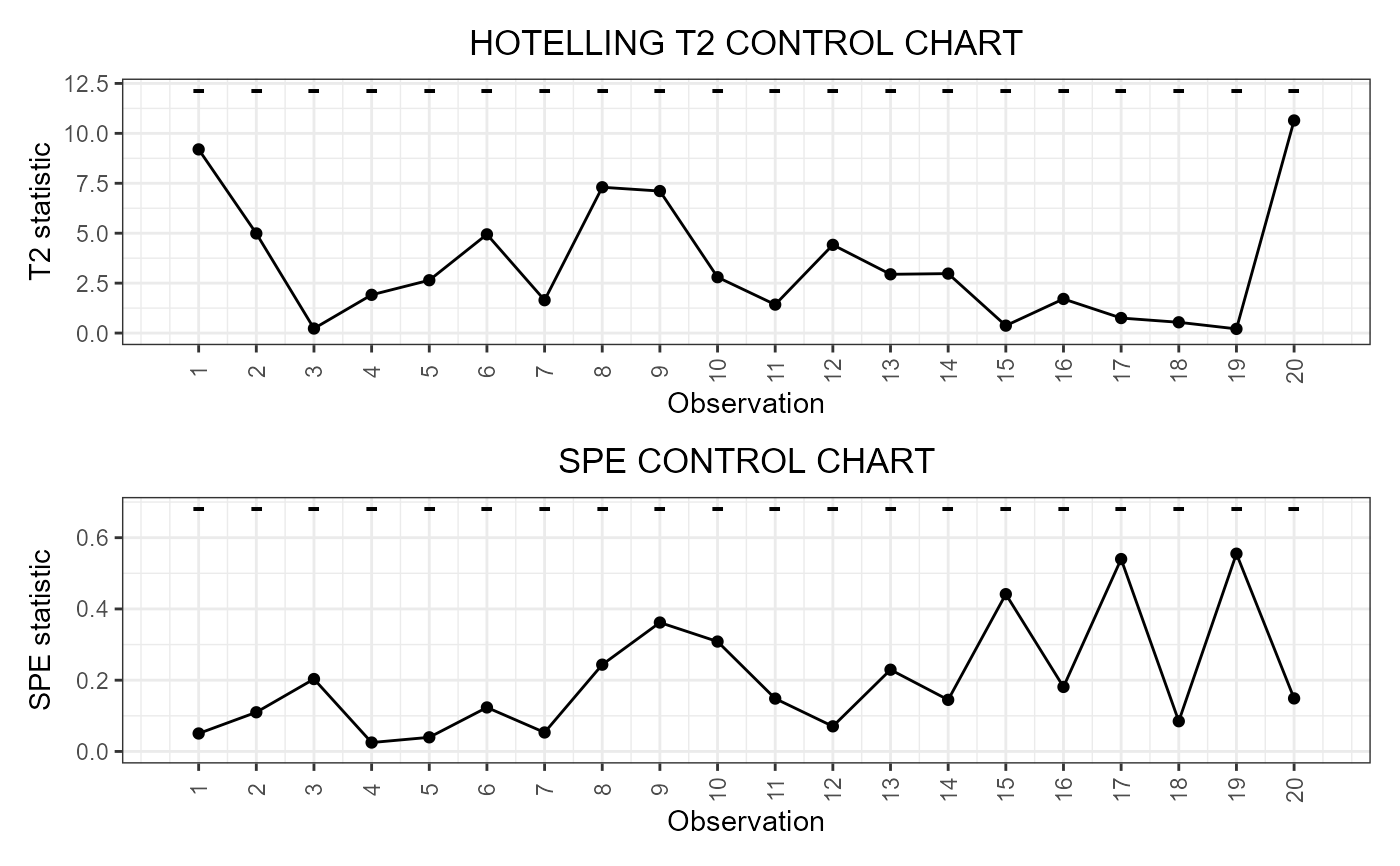
This function builds a data frame needed to plot the Hotelling's T2 and squared prediction error (SPE) control charts based on multivariate functional principal component analysis (MFPCA) performed on multivariate functional data, as Capezza et al. (2020) for the multivariate functional covariates. The training data have already been used to fit the model. An optional tuning data set can be provided to estimate the control chart limits. A phase II data set contains the observations to be monitored with the control charts.

control_charts_pca(
  pca,
  components = NULL,
  tuning_data = NULL,
  newdata,
  alpha = 0.05,
  limits = "standard",
  seed,
  nfold = 5,
  ncores = 1,
  tot_variance_explained = 0.9,
  single_min_variance_explained = 0,
  absolute_error = FALSE
)

Arguments

pca

An object of class pca_mfd obtained by doing MFPCA on the training set of multivariate functional data.

components

A vector of integers with the components over which to project the multivariate functional data. If this is not NULL, the arguments `single_min_variance_explained` and `tot_variance_explained` are ignored. If NULL, components are selected such that the total fraction of variance explained by them is at least equal to the argument `tot_variance_explained`, where only components explaining individually a fraction of variance at least equal to the argument `single_min_variance_explained` are considered to be retained. Default is NULL.

tuning_data

An object of class mfd containing the tuning set of the multivariate functional data, used to estimate the T2 and SPE control chart limits. If NULL, the training data, i.e. the data used to fit the MFPCA model, are also used as the tuning data set, i.e. tuning_data=pca$data. Default is NULL.

newdata

An object of class mfd containing the phase II set of the multivariate functional data to be monitored.

alpha

If it is a number between 0 and 1, it defines the overall type-I error probability and the Bonferroni correction is applied by setting the type-I error probability in the two control charts equal to alpha/2. If you want to set manually the Type-I error probabilities in the two control charts, then the argument alpha must be a named list with two elements, named T2 and spe, respectively, each containing the desired Type I error probability of the corresponding control chart. Default value is 0.05.

limits

A character value. If "standard", it estimates the control limits on the tuning data set. If "cv", the function calculates the control limits only on the training data using cross-validation using calculate_cv_limits. Default is "standard".

seed

If limits=="cv", since the split in the k groups is random, you can fix a seed to ensure reproducibility. Deprecated: use set.seed() before calling the function for reproducibility.

nfold

If limits=="cv", this gives the number of groups k used for k-fold cross-validation. If it is equal to the number of observations in the training data set, then we have leave-one-out cross-validation. Otherwise, this argument is ignored.

ncores

If limits=="cv", if you want perform the analysis in the k groups in parallel, give the number of cores/threads. Otherwise, this argument is ignored.

tot_variance_explained

The minimum fraction of variance that has to be explained by the set of multivariate functional principal components retained into the MFPCA model fitted on the functional covariates. Default is 0.9.

single_min_variance_explained

The minimum fraction of variance that has to be explained by each multivariate functional principal component such that it is retained into the MFPCA model. Default is 0.

absolute_error

If FALSE, the SPE statistic, which monitors the principal components not retained in the MFPCA model, is calculated as the sum of the integrals of the squared prediction error functions, obtained as the difference between the actual functions and their approximation after projection over the selected principal components. If TRUE, the SPE statistic is calculated by replacing the square of the prediction errors with the absolute value, as proposed by Capizzi and Masarotto (2018). Default value is FALSE.

Value

A data.frame with as many rows as the number of multivariate functional observations in the phase II data set and the following columns:

* one id column identifying the multivariate functional observation in the phase II data set,

* one T2 column containing the Hotelling T2 statistic calculated for all observations,

* one column per each functional variable, containing its contribution to the T2 statistic,

* one spe column containing the SPE statistic calculated for all observations,

* one column per each functional variable, containing its contribution to the SPE statistic,

* T2_lim gives the upper control limit of the Hotelling's T2 control chart,

* one contribution_T2_*_lim column per each functional variable giving the limits of the contribution of that variable to the Hotelling's T2 statistic,

* spe_lim gives the upper control limit of the SPE control chart

* one contribution_spe*_lim column per each functional variable giving the limits of the contribution of that variable to the SPE statistic.

References

Capezza C, Lepore A, Menafoglio A, Palumbo B, Vantini S. (2020) Control charts for monitoring ship operating conditions and CO2 emissions based on scalar-on-function regression. Applied Stochastic Models in Business and Industry, 36(3):477--500. <doi:10.1002/asmb.2507>

Capizzi, G., & Masarotto, G. (2018). Phase I distribution-free analysis with the R package dfphase1. In Frontiers in Statistical Quality Control 12 (pp. 3-19). Springer International Publishing.

See also

regr_cc_fof

Examples

library(funcharts)
data("air")
air <- lapply(air, function(x) x[1:220, , drop = FALSE])
fun_covariates <- c("CO", "temperature")
mfdobj_x <- get_mfd_list(air[fun_covariates],
                         n_basis = 15,
                         lambda = 1e-2)
y <- rowMeans(air$NO2)
y1 <- y[1:100]
y_tuning <- y[101:200]
y2 <- y[201:220]
mfdobj_x1 <- mfdobj_x[1:100]
mfdobj_x_tuning <- mfdobj_x[101:200]
mfdobj_x2 <- mfdobj_x[201:220]
pca <- pca_mfd(mfdobj_x1)
cclist <- control_charts_pca(pca = pca,
                             tuning_data = mfdobj_x_tuning,
                             newdata = mfdobj_x2)
plot_control_charts(cclist)